AMS-Climate Model
Goal:
Overlay the trends of the CSIRO Global Climate Model Mk 3.5 - Scenario SRESA2 (http://www.marine.csiro.au/marq/edd_search.Browse_Citation?txtSession=7024) data over the existing AMS forcing temperature and salinity data.
Step1 - Match up the AMS layers in the water column with the climate depth bins.
There were a number of possible ways to do this.
- Calculate averages of all bins in layers.
- Use data from the closest layer
We have selected option 2. We are just finding the closest layer in the climate model to the AMS depth values.
Find the average value of the climate data in each AMS polygon.
for each box
if number of climate data point in box > 0
for each layer
find average value from climate data in this box in this layer
end
% deal with boxes where there is no climate data within polygon
% here we take the average of the average value calculated in the adjacent loop. Note this does not use the raw climate data in the adjacent polygons but the value that has been calculated in the previous step.
Step3:
Applying the calculated climate trends to the existing AMS temperature and salinity files.
The existing AMS forcing files contain data from 1991-1995 generated by the bluelink model. This data is then cycled through each 5 years.
As you can see from the graph below there is alot of variation in the 5 years worth of Data.
So we have bluelink data from 1991 - 1995 and then climate trend data (calculated using the above algorithm) from 2001-2050.
We need to ‘overlay’ the trend data on the existing bluelink data.
There are a number of options for doing this:
Continue cycling through the 5 years worth of bluelink data and overlay the new climate trend data to get a new dataset that is 1991 - 2050.
Pick a ‘representative’ year from the bluelink data and overlay the climate trend data to that.
Create a new average year worth of bluelink data and then overlay the climate trend data to that.
We have selected option 3 and we will create a new data set from 1991 - 2050 where the climate data is overlaid from 2001-2050.
Sample output:
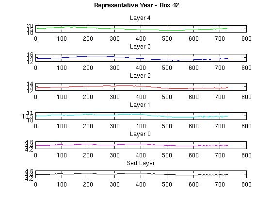
These are the plots for box 42:
The ‘representative’ year. This is the original AMS temperature forcing file averaged over the 5 years of data. This should hopefully contain seasonal information but not have the issues of the original data with the changes between each year.
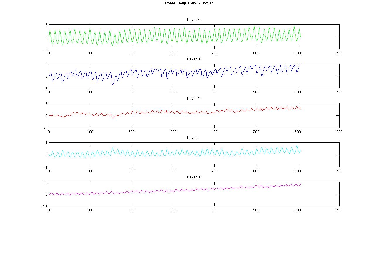
This plot shows the temperature trend data extracted from the CSIRO climate model.
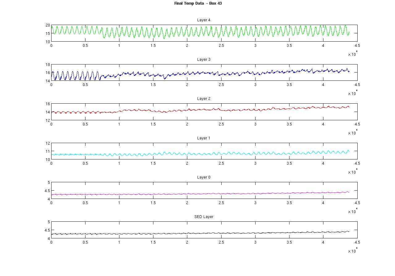
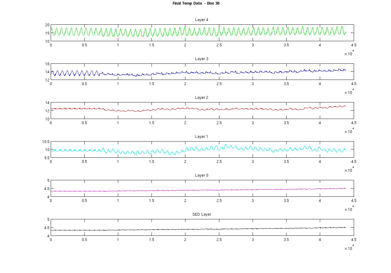
This plot is the final temperature dataset for box 42.
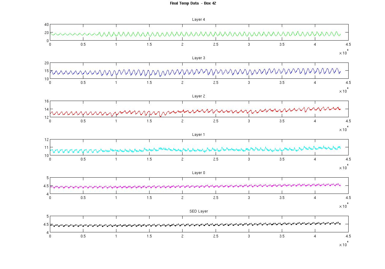
Discussion:
Each of the plots show the temperature data for each of the layers in the file with the top subplot the surface layer down to the bottom water column layer and the sediment layer (which has the same value as the bottom layer in the forcing files).
As you can see from the first plot the way we are calculating the ‘trend’ in the climate data also includes the interannual trends. As these are basically added to the interannual trends of the existing data the signal is amplified.
Ideally we would change our method of calculating the climate trend to smooth out the seasonal signal without removing any changes in the seasonal signal due to climate change.
Filtered data
To get rid of the amplification of the seasonal signal from the combined AMS ‘rep’ year data and the climate trend data we decided to try to filter out the seasonal signal from either the climate trend data or the ‘rep’ AMS data. There is really only a seasonal trend in the original temperature AMS data - the salinity data doesn’t need to be filtered as there is no amplification of the seasonal signal.
Filtering the temperature trend data
Here we are removing the seasonal trend from the temperature trend data before it is added to the AMS rep year data.
The following figure shows the typical frequency response of the temperature trend data in a surface box.
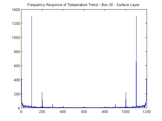
As you can see there is a strong artifact around the 100 mark - this is the seasonal component. So if we filter this out we get a trend signal without the seasonal component.
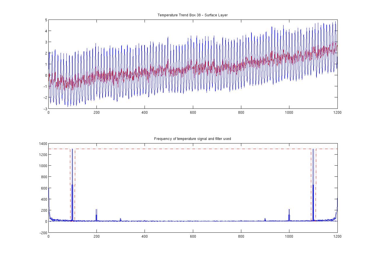
The following figure shows the temperature trend before and after filtering with the frequency response and filter design in the bottom plot.
This filter design is a bandStop filter - we are just filtering out the seasonal frequency.
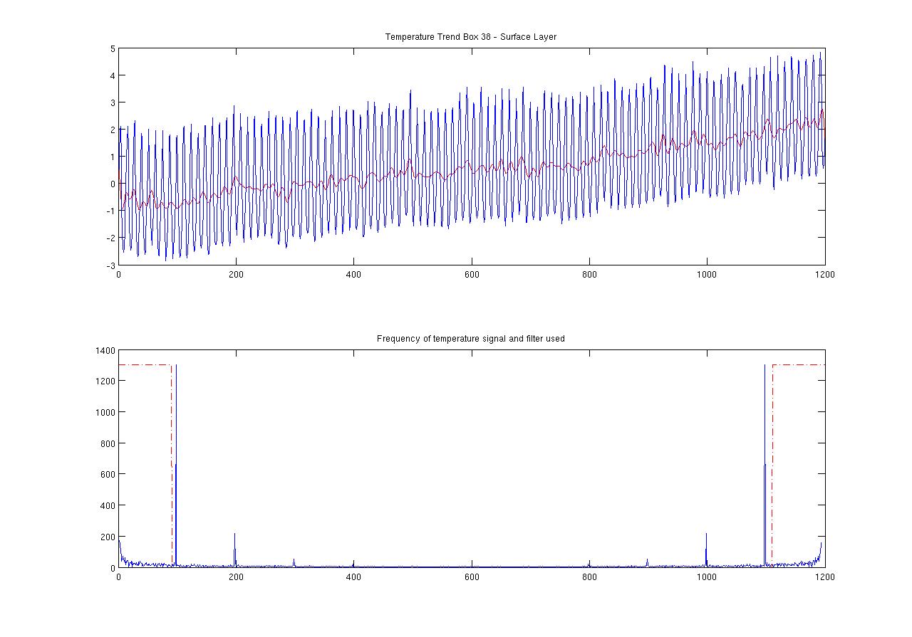
The following figure shows the outcome when we use a lowpass filter - here we are filtering out any frequencies above the seasonal frequency. This gives a ‘smoother’ results but we might be loosing higher frequency changes.
Advantages:
As we are using the original AMS temperature and salinity data unfiltered we will keep any spatial variation in the seasonal trend that is present in this data.
Disadvantages:
We will probably loose the seasonal variation in the climate data.
Filtering the ‘rep’ AMS data.
The representative year is calculated by averaging the original AMS over 1991 - 1995. This gives us a single year worth of data.
This is then filtered to remove the seasonal trend similar to how we are filtering above.
Advantages:
We keep the seasonal trend in the climate data.
We we don’t need to filter the salinity data we can use the generated climate trend salinity data and just overlay the original AMS salinity data. If we remove the seasonal trend in the AMS temperature data and then overlay unfiltered climate temperature trend data we will keep the climate seasonal data.
Disadvantages:
We will loose any seasonal spatial variation in the original AMS temperature data.
Final sample plots: